[代码实践] 手写 ICP/NDT 配准算法性能比较

介绍

关于 ICP 和 NDT 的算法原理可以参考：激光 SLAM 点云配准 - 基于 ICP 及其变种的方法，激光SLAM 点云配准 - 基于相关性的方法。这篇博客主要整理 ICP 的实现过程，以及最后和 PCL 库自带的 ICP 和 NDT 算法接口进行比较。测试框架是基于任乾大佬的 localization_in_auto_driving 进行魔改 :)。主要是为了方便在同一个环境下测试各类算法效果。代码在：General Mapping and Localization Framework

基于 SVD 分解进行 ICP 配准

算法原理可以参考之前写的博客，这里直接列出相关代码：

/// 设置 ICP 匹配参数，主要包括：最大关联距离，相邻两次迭代间的最大接收位姿变化程度以及匹配得分变化，以及最大迭代次数
bool ICPRegistration::SetRegistraionParam(float max_correspodence_dist,
                                          float trans_eps,
                                          float fitness_eps,
                                          int max_iter) {
    param_.max_correspodence_dist = max_correspodence_dist;
    param_.trans_eps = trans_eps;
    param_.fitness_eps = fitness_eps;
    param_.max_iter = max_iter;

    return true;
}

/// 设置匹配目标点云，用于建立 KD 树方便后续快速搜索最近点
bool ICPRegistration::SetInputTarget(const CloudData::Cloud_Ptr& input_target) {

    target_kd_tree_ptr_->setInputCloud(input_target);
    return true;
}

/// 进行 SVD 分解进行 ICP 配准，获得两个点云之间的相对位姿变化
bool ICPRegistration::MatchWithSVD(const CloudData::Cloud_Ptr& input_source,
                                   const Eigen::Matrix4f& predict_pose,
                                   Eigen::Matrix4f& result_pose)

{
    Eigen::Matrix4f esitimated_pose = predict_pose;
    bool converge = false;
    int iter = 0;

    // keep updating pose until converge or reach max iteration
    while (iter < param_.max_iter && !converge) {
        iter++;

        CloudData::Cloud transformed_cloud;
        pcl::transformPointCloud(*input_source, transformed_cloud, esitimated_pose);

        std::vector<float> source_points_xyz;
        std::vector<float> target_points_xyz;
        
        // 预留足够空间，避免频繁空间分配
        source_points_xyz.reserve(transformed_cloud.points.size() * 3);
        target_points_xyz.reserve(transformed_cloud.points.size() * 3);

        // 循环的过程同时计算上一次迭代最后的每个点平均关联距离
        float score = 0.0;
        for (size_t i = 0; i < input_source->points.size(); ++i) {
            const CloudData::Point& transformed_point = transformed_cloud.points[i];

            std::vector<int> indices(1);
            std::vector<float> distances(1);

            target_kd_tree_ptr_->nearestKSearch(transformed_point, 1, indices, distances);

            score += distances[0];

            if (distances[0] > param_.max_correspodence_dist) continue;

            source_points_xyz.push_back(input_source->points[i].x);
            source_points_xyz.push_back(input_source->points[i].y);
            source_points_xyz.push_back(input_source->points[i].z);

            target_points_xyz.push_back(target_kd_tree_ptr_->getInputCloud()->points[indices[0]].x);
            target_points_xyz.push_back(target_kd_tree_ptr_->getInputCloud()->points[indices[0]].y);
            target_points_xyz.push_back(target_kd_tree_ptr_->getInputCloud()->points[indices[0]].z);
        }

        // condition 1: fitness score converge -- 匹配距离收敛
        score /= (transformed_cloud.points.size());
        if (std::fabs(score_ - score) < param_.fitness_eps) {
            converge = true;
            break;
        }
        score_ = score;

        // 使用 Eigen::Map 来避免多余空间使用
        Eigen::Map<Eigen::Matrix3Xf> source_points(source_points_xyz.data(), 3, source_points_xyz.size() / 3);
        Eigen::Map<Eigen::Matrix3Xf> target_points(target_points_xyz.data(), 3, target_points_xyz.size() / 3);

        Eigen::Vector3f source_mean = source_points.rowwise().mean();
        Eigen::Vector3f target_mean = target_points.rowwise().mean();

        source_points.colwise() -= source_mean;
        target_points.colwise() -= target_mean;

        Eigen::Matrix3f H = source_points * target_points.transpose();
        Eigen::JacobiSVD<Eigen::Matrix3f> svd(H, Eigen::ComputeFullU | Eigen::ComputeFullV);

        Eigen::Vector3f prev_translation = esitimated_pose.block<3, 1>(0, 3);

        Eigen::Matrix3f updated_rotation = svd.matrixV() * svd.matrixU().transpose();
        Eigen::Vector3f updated_translation = target_mean - updated_rotation * source_mean;

        esitimated_pose.block<3, 3>(0, 0) = updated_rotation;
        esitimated_pose.block<3, 1>(0, 3) = updated_translation;

        // condition 2: translation converge -- 这里只比较了平移没有考虑旋转的变化程度
        if ((updated_translation - prev_translation).squaredNorm() < param_.trans_eps) {
            converge = true;
        }
    }
    result_pose = esitimated_pose;

    return true;
}

基于高斯牛顿法进行 ICP 配准

高斯牛顿法和过程和 SVD 大同小异，区别在于不适用 SVD 分解获得最优估计位姿，而是通过高斯牛顿法尝试取降低匹配残差。这里对每一个点的残差函数为：

$$
\boldsymbol{e} = \boldsymbol{Rp}_i + \boldsymbol{t} - \boldsymbol{p}'_i
$$

其中， $\boldsymbol{R}, \boldsymbol{t}$ 为当前帧相对于匹配目标（上一帧点云或者局部地图）的位姿， $\boldsymbol{p}_i$ 为当前帧点云中的一个点， $\boldsymbol{p}'_i$ 为匹配目标中和 $\boldsymbol{p}$ 关联的一个点，这里我们取最近点作为关联点。

根据高斯牛顿法需要求出残差对优化变量（ $\boldsymbol{R}, \boldsymbol{t}$ ）的雅可比矩阵，对旋转矩阵使用右扰动模型求解，推导过程参考：一些常见的关于旋转的函数对旋转求导过程的推导，下面直接给出结果：

$$
\begin{aligned}
    \frac{\partial\boldsymbol{e}_i}{\partial\boldsymbol{R}} &= -\boldsymbol{Rp}^\wedge\\
    \frac{\partial\boldsymbol{e}_i}{\partial\boldsymbol{t}} &= \boldsymbol{I}\\
    \boldsymbol{J}_i &= \begin{bmatrix}
        \frac{\partial\boldsymbol{e}_i}{\partial\boldsymbol{R}} & \frac{\partial\boldsymbol{e}_i}{\partial\boldsymbol{t}}
    \end{bmatrix} \in \mathbb{R}^{3\times 6}
\end{aligned}
$$

因此，正规方程（Normal Equation）为：

$$
\begin{aligned}
    \boldsymbol{H}\delta\boldsymbol{x} &= \boldsymbol{b}\\
    \boldsymbol{H} &= \sum_{i}\boldsymbol{J}_i^T\boldsymbol{J}_i \in \mathbb{R}^{6\times6}\\
    \boldsymbol{b} &= -\sum_{i}\boldsymbol{J}_i^T\boldsymbol{e}_i \in \mathbb{R}^{6\times1}
\end{aligned}
$$

求解正规方程，对状态量进行迭代即可，这里注意由于我们使用的是右扰动模型求解，因此更新旋转时也应该右乘迭代量：

$$
\begin{aligned}
    \boldsymbol{R}' &= \boldsymbol{R}\exp{(\delta\boldsymbol{x}_{0:2})}\\
    \boldsymbol{t}' &= \boldsymbol{t} + \delta\boldsymbol{x}_{3:5}
\end{aligned}
$$

高斯牛顿法和参数设置和目标设置代码和 SVD 一样，这里只列出核心匹配函数：

bool ICPRegistration::MatchWithGassianNewton(const CloudData::Cloud_Ptr& input_source,
                                             const Eigen::Matrix4f& predict_pose,
                                             Eigen::Matrix4f& result_pose) {
    Eigen::Matrix4f esitimated_pose = predict_pose;
    bool converge = false;
    int iter = 0;

    // keep updating pose until converge or reach max iteration
    while (iter < param_.max_iter && !converge) {
        iter++;

        CloudData::Cloud transformed_cloud;
        pcl::transformPointCloud(*input_source, transformed_cloud, esitimated_pose);

        // 初始化 H, b
        Eigen::Matrix<float, 6, 6> H = Eigen::Matrix<float, 6, 6>::Zero();  // J^TJ
        Eigen::Matrix<float, 6, 1> b = Eigen::Matrix<float, 6, 1>::Zero();  // J^Te

        // 对每个点计算在目标点云中的最近点，计算其雅可比和残差，构建 H，b
        float score = 0.0;
        for (size_t i = 0; i < input_source->points.size(); ++i) {
            const CloudData::Point& transformed_point = transformed_cloud.points[i];

            std::vector<int> indices(1);
            std::vector<float> distances(1);

            target_kd_tree_ptr_->nearestKSearch(transformed_point, 1, indices, distances);

            const CloudData::Point& original_point = input_source->points[i];
            const CloudData::Point& nearest_point = target_kd_tree_ptr_->getInputCloud()->points[indices[0]];
            score += distances[0];

            if (distances[0] > param_.max_correspodence_dist) continue;

            Eigen::Vector3f source_pt(original_point.x, original_point.y, original_point.z);
            Eigen::Vector3f transformed_pt(transformed_point.x, transformed_point.y, transformed_point.z);
            Eigen::Vector3f target_pt(nearest_point.x, nearest_point.y, nearest_point.z);

            // 计算雅可比矩阵
            Eigen::Matrix<float, 3, 6> jacobian = Eigen::Matrix<float, 3, 6>::Zero();
            jacobian.block<3, 3>(0, 0) = -esitimated_pose.block<3, 3>(0, 0) * Sophus::SO3f::hat(source_pt);
            jacobian.block<3, 3>(0, 3) = Eigen::Matrix3f::Identity();
            // 计算残差
            Eigen::Vector3f resiual = transformed_pt - target_pt;

            // 更新 H, b
            H += jacobian.transpose() * jacobian;
            b += -jacobian.transpose() * resiual;
        }

        // condition 1: fitness score converge
        score /= (transformed_cloud.points.size());
        if (std::fabs(score_ - score) < param_.fitness_eps) {
            converge = true;
            break;
        }
        score_ = score;
        
        // 求解 Hx = b
        Eigen::Matrix<float, 6, 1> delta_x = H.householderQr().solve(b);

        // 更新 R, t
        esitimated_pose.block<3, 3>(0, 0) *= Sophus::SO3f::exp(delta_x.block<3, 1>(0, 0)).matrix();
        esitimated_pose.block<3, 1>(0, 3) += delta_x.block<3, 1>(3, 0);

        // condition 2: transformation converge
        if (delta_x.squaredNorm() < param_.trans_eps) {
            converge = true;
        }
    }

    // used final mean distance (across all points) as fitness score
    result_pose = esitimated_pose;

    return true;
}

PCL 库中的 ICP，NDT 接口

PCL 库中也自带了 ICP 和 NDT 的算法接口，下面简单介绍一下如何使用。

PCL-ICP

大致来说也是分成四步：参数设置，目标设置，点云配准以及获取匹配残差，如下：

// 初始化 ICP 接口
icp_ptr_.reset(new pcl::IterativeClosestPoint<CloudData::Point, CloudData::Point>());

// 参数设置
icp_ptr_->setMaxCorrespondenceDistance(max_correspodence_dist);
icp_ptr_->setMaximumIterations(max_iter);
icp_ptr_->setTransformationEpsilon(trans_eps);
icp_ptr_->setEuclideanFitnessEpsilon(fitness_eps);

// 目标点云设置
// CloudData::Cloud_Ptr input_target; 获取目标点云，可以是上一帧点云，或者其他形式的点云地图
icp_ptr_->setInputTarget(input_target);

// 点云配准，获取匹配结果
// input_source (用来匹配的点云，通常是最新一帧点云)
// Eigen::Matrix4f predict_pose 预测位姿（初始值）
// CloudData::Cloud_Ptr result_cloud_ptr // 使用 ICP 估计后的位姿转换的匹配点云
// Eigen::Matrix4f result_pose ICP 最终位姿估计
icp_ptr_->setInputSource(input_source);
icp_ptr_->align(*result_cloud_ptr, predict_pose);
result_pose = icp_ptr_->getFinalTransformation();
score_ = icp_ptr_->getFitnessScore();   // 最后匹配残差（所有关联点对的平均距离）

PCL-NDT

PCL 库中的 NDT 和 ICP 接口基本类似，如下所示：

// 初始化 NDT 接口
ndt_ptr_.reset(new pcl::NormalDistributionsTransform<CloudData::Point, CloudData::Point>());

// 参数设置，包括分辨率，迭代步长等
ndt_ptr_->setResolution(res);
ndt_ptr_->setStepSize(step_size);
ndt_ptr_->setTransformationEpsilon(trans_eps);
ndt_ptr_->setMaximumIterations(max_iter);

// 目标点云设置
// CloudData::Cloud_Ptr input_target; 获取目标点云，可以是上一帧点云，或者其他形式的点云地图
ndt_ptr_->setInputTarget(input_target);

// 点云配准，获取匹配结果
// input_source (用来匹配的点云，通常是最新一帧点云)
// Eigen::Matrix4f predict_pose 预测位姿（初始值）
// CloudData::Cloud_Ptr result_cloud_ptr // 使用 ICP 估计后的位姿转换的匹配点云
// Eigen::Matrix4f result_pose ICP 最终位姿估计
ndt_ptr_->setInputSource(input_source);
ndt_ptr_->align(*result_cloud_ptr, predict_pose);
result_pose = ndt_ptr_->getFinalTransformation();
ndt_ptr_->getFitnessScore();  // 最后匹配残差（所有关联点对的平均距离）

测试

接下来以 KITTI 数据集为例进行简单的测试，匹配大致流程为：

第一帧不进行匹配，初始化局部地图
在局部地图累计若干帧之前不对点云进行下采样，直接将点云转换至世界坐标系中加入局部地图
每一帧通过和局部地图进行匹配获得相对位姿变换，并计算其世界坐标
每一帧点云的初始位姿预测值，为上一帧点云的世界坐标与上一帧估计的相对位姿变化（即假设载体在进行匀速运动，因此每两帧之间的相对运动基本保持不变）

最后使用 EVO 将里程计获得的位姿和真值（GNSS）进行比较。

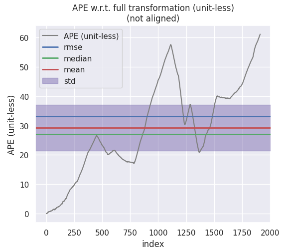
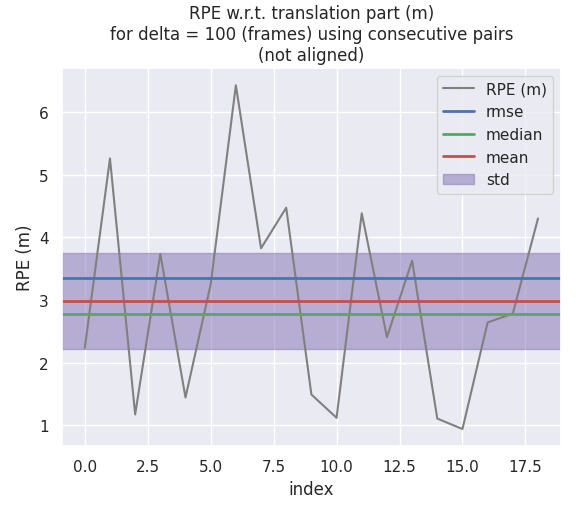
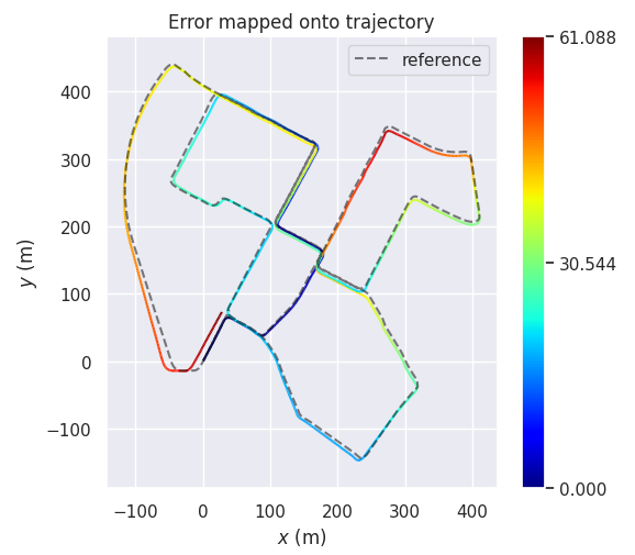
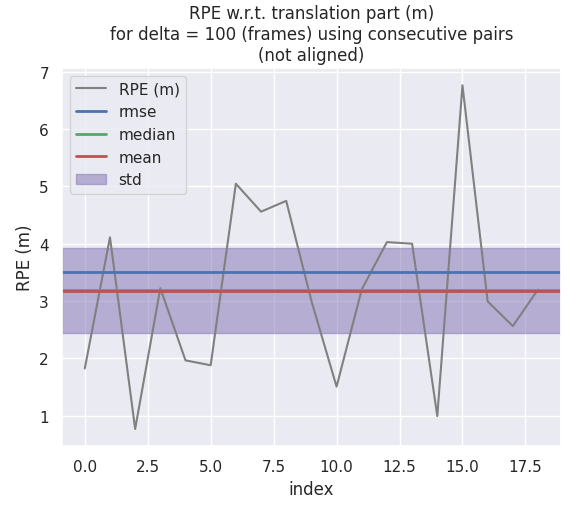
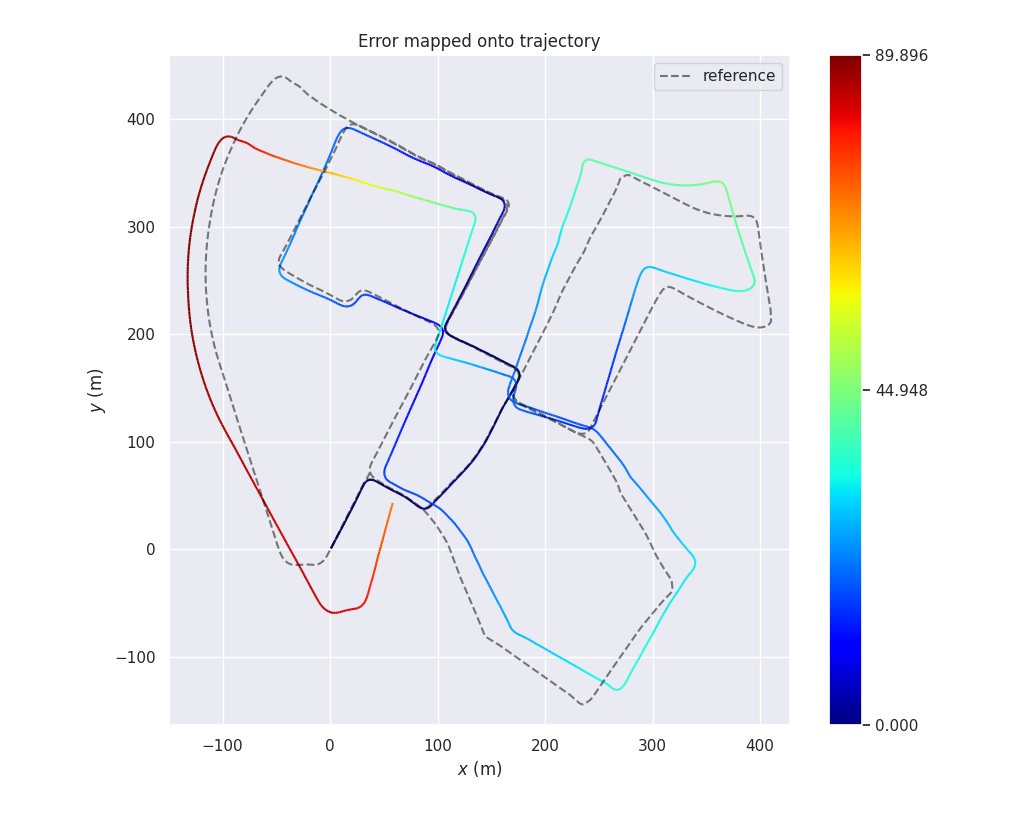
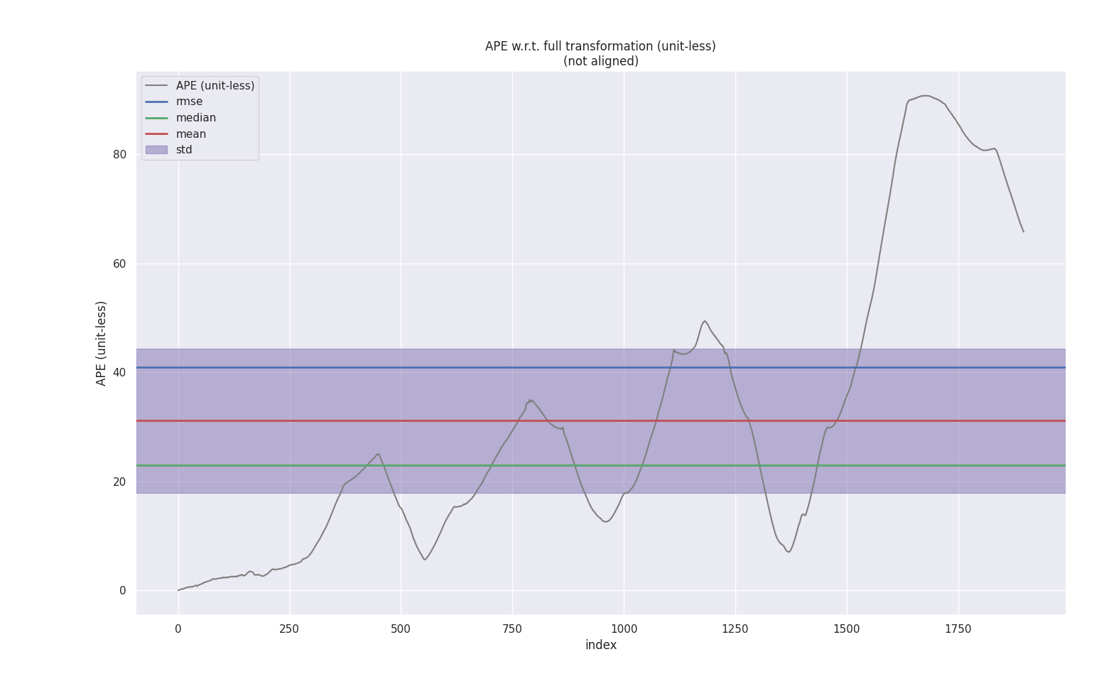
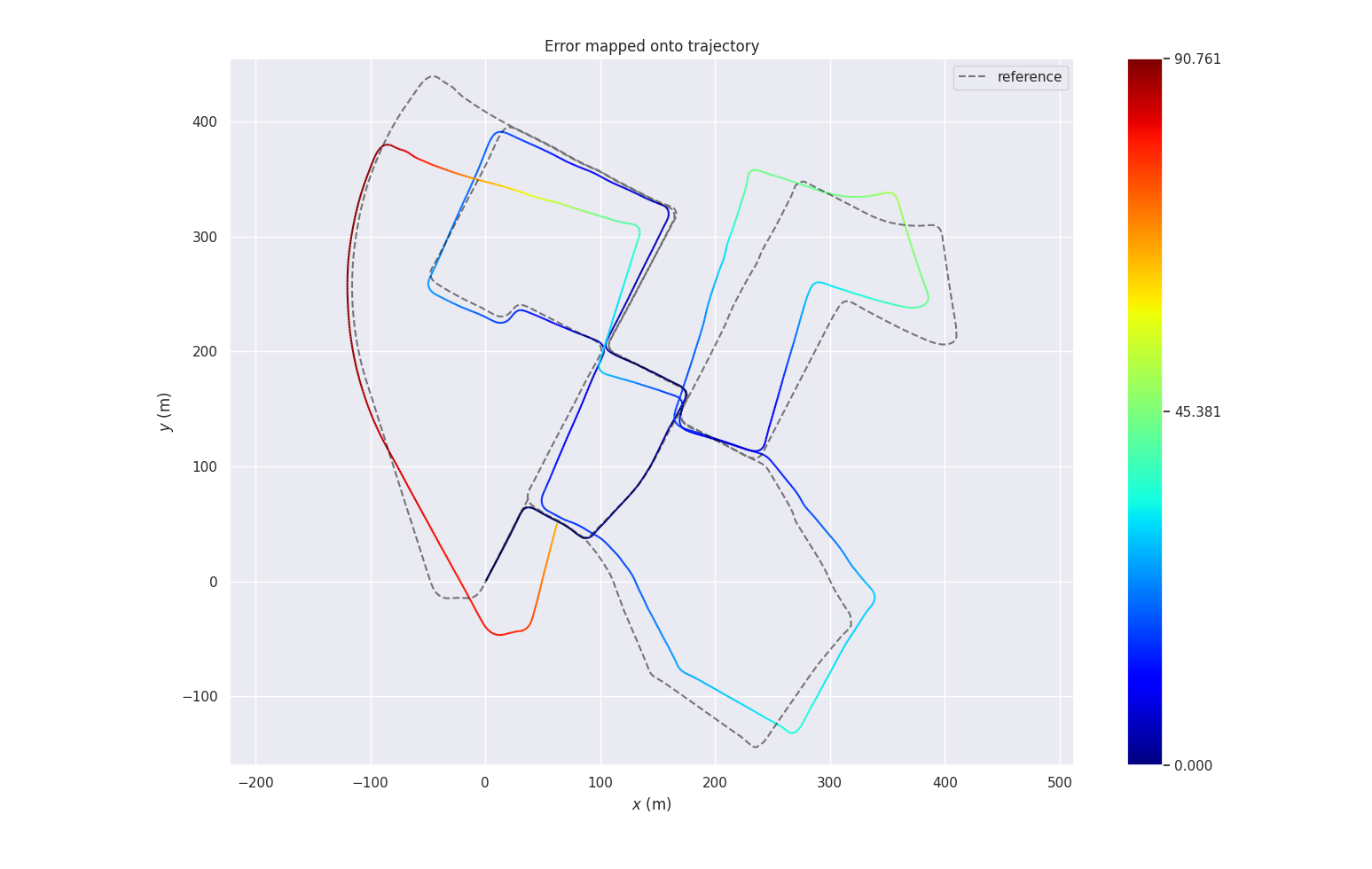
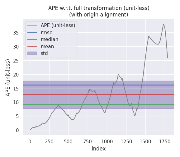
PCL-NDT

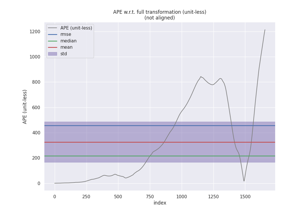
绝对位姿误差（APE）

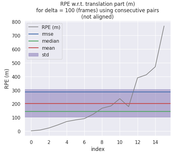
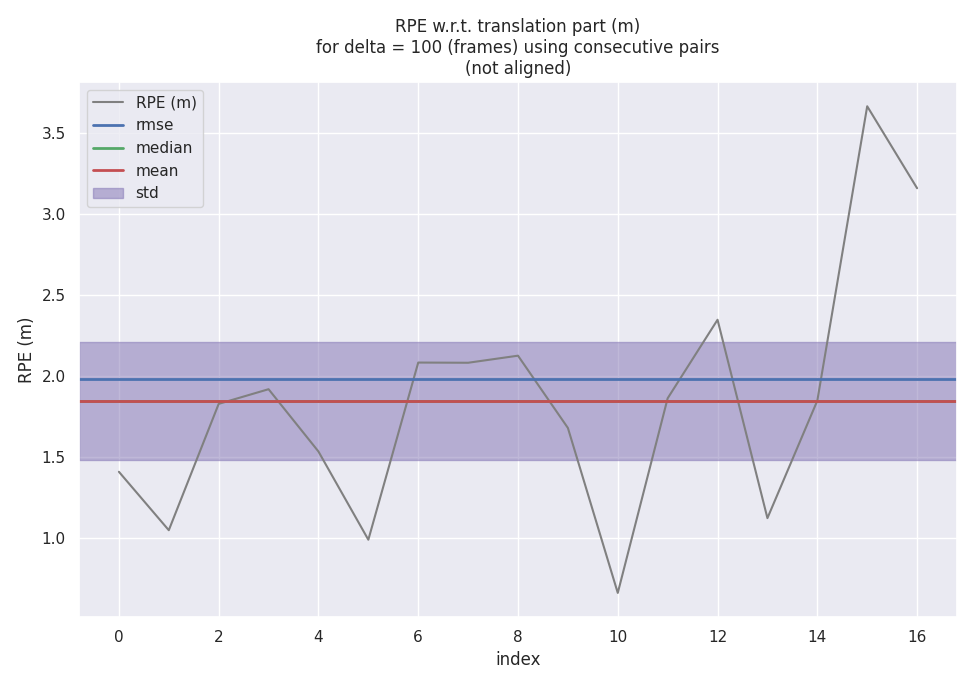
相对位姿误差（RPE）

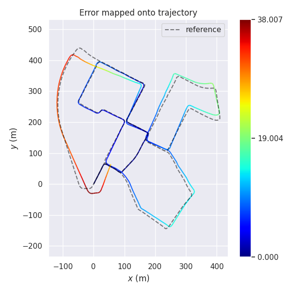
轨迹比较

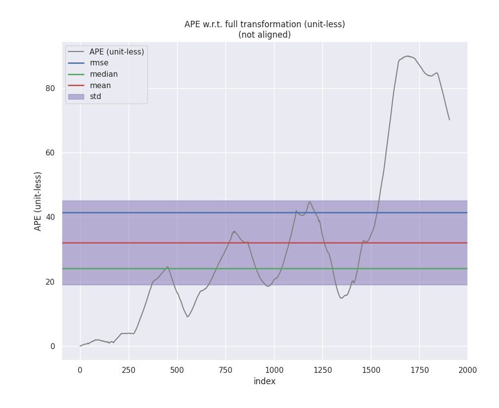
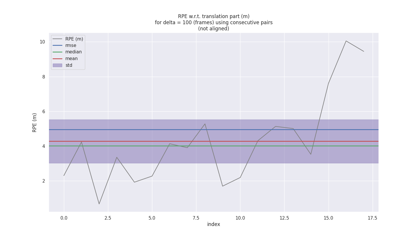
SVD-ICP

绝对位姿误差（APE）

相对位姿误差（RPE）

轨迹比较

GN-ICP

绝对位姿误差（APE）

相对位姿误差（RPE）

轨迹比较

PCL-ICP

绝对位姿误差（APE）

相对位姿误差（RPE）

轨迹比较

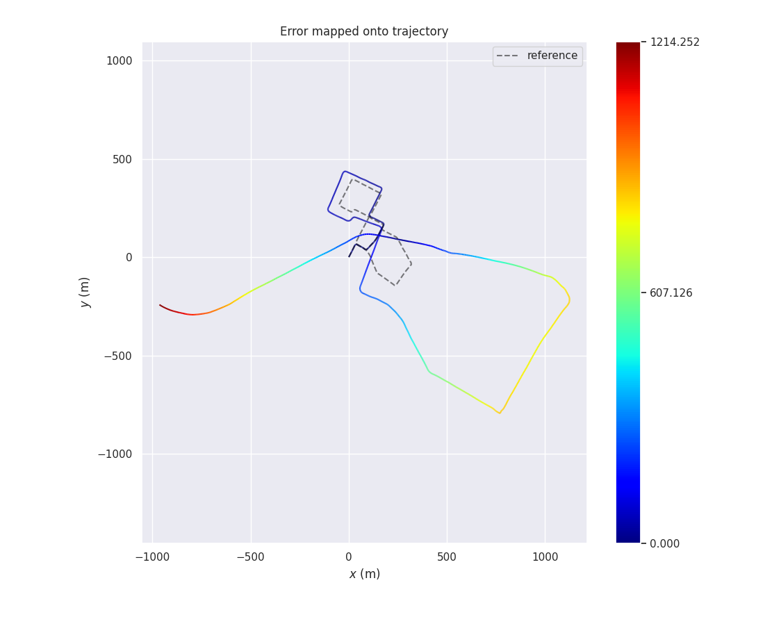
A-LOAM

在测试传统的 ICP/NDT 算法之后，想顺便比较一下基于 LOAM 系列的里程计的性能如何，于是乎简单将 A-LOAM 的输出也进行相似的比较，EVO 比较结果如下。不难看出，从各个参数来看基于 A-LOAM 的里程计都由于基于传统点云配准方法，当然 A-LOAM 本身输出的位姿也已经经过后端的优化，所以也能起到一定的校正作用。

绝对位姿误差（APE）

相对位姿误差（RPE）

轨迹比较

性能比较

首先说明的是，这个比较并不能说明哪种算法一定表现会更好，而只是针对某个测试集进行简单的定性测试。另外，从图也能看出，PCL 库中的 ICP 定位到最后漂移失败导致里程计崩溃了，这个目前不太清楚是什么原因，查了一下发现其他博主貌似也有类似的结论，因此考虑可能是 PCL 库中的 ICP 算法有 Bug，因此下面主要比较自己写的两个 ICP 算法以及 PCL 库中的 NDT 算法。

从绝对误差来看的话，NDT 性能最好，基于 SVD 和 GN 实现的 ICP 性能差别不大，此外观察以下可以看到，在前期三种的算法的精度都差不太多，是在某一处转弯之后出现了一点较大的漂移导致后面轨迹的发散。

评价里程计的漂移使用相对轨迹误差可能会更好一点，从相对轨迹误差误差来看的话，NDT 和 SVD-ICP 差别不大，而 GN-ICP 在最后有发散的迹象。

此外我还记录了每一种算法的平均耗时，NDT，SVD-ICP，GN-ICP 的平均耗时分别为：14.2579 ms, 17.9568 ms, 18.154 ms。NDT 和 ICP 之间的比较意义不太大（参数不一致），而 GN-ICP 的平均耗时略高于 SVD-ICP （5% 左右）。