简介
在之前的博客中 (G2O 学习记录(一)),我结合 2D 激光 SLAM 简单介绍了一下 G2O 库的基本用法,这篇博客主要是在 3D 激光 SLAM 框架中基于 G2O 实现激光里程计,GNSS 以及回环约束在 KITTI 数据集下进行图优化。
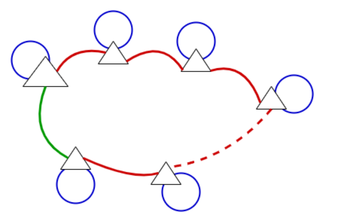
简单介绍了一下优化过程中涉及的节点和边。首先是节点,由于是纯激光 SLAM (没有 IMU 和视觉等),因此优化变量只有载体的位姿。因此这个图也是个位姿图。边包括三种:激光里程计产生的前后两帧的相对位姿约束,GNSS 对位姿节点的先验约束以及回环检测产生的轨迹中形成回环的两帧的相对位姿约束。如下图所示,三角形为载体位姿,红边为激光里程计对相邻两帧的位姿约束,蓝边为 GNSS 对某一帧的的位置约束(不包含姿态),绿边为回环检测到的某两帧之间的位姿约束。
关于非线性优化的原理可以参考:最小二乘问题和非线性优化。在这个问题中,图优化需要做到以下几步:
- 添加节点(位姿)和边(位姿或位置约素)为优化做准备
- 优化过程,对每条边计算误差以及对优化变量的雅可比矩阵,这里的边有两个类型(两帧节点之间的相对位姿观测,以及对单个节点的位置观测),我们需要对这两种边的误差以及雅可比计算方式进行推导
- 选择合适的优化策略,如 LM 或者 Dogleg 法,利用每个观测的误差和雅可比矩阵构建正规方程
$\boldsymbol{H}\Delta\boldsymbol{x} = \boldsymbol{b}$ - 对上述方程选择合适的方式进行求解,例如 QR 分解、Cholesky 分解等
- 按照需要添加鲁棒核函数,不过这里基本都是位姿之间的约束,不涉及特征,因此误匹配的情况应该比较少
接下来看 G2O 如何实现上述过程。
节点和边的选择
和 Ceres Solver 不同,G2O 作为专门用于进行图优化的库,提供了大量预先定义的节点和边供用户调用,在这个实践中主要涉及一种节点和两个边,分别是 VertexSE3(位姿节点),EdgeSE3 (对两个位姿节点的约束边),EdgeSE3XYZPrior (对一个位姿节点的先验边),下面分别来看一下:
VertexSE3 结构
先看位姿节点的定义:
  class G2O_TYPES_SLAM3D_API VertexSE3 : public BaseVertex<6, Isometry3>
  {
    public:
      // 内存对齐
      EIGEN_MAKE_ALIGNED_OPERATOR_NEW;

      // 在进行 1000 次更新后重新进行正交化
      static const int orthogonalizeAfter = 1000; //< orthogonalize the rotation matrix after N updates

      VertexSE3();

      // 将估计值设为原点,这里设为单位帧
      virtual void setToOriginImpl() {
        _estimate = Isometry3::Identity();
      }

      // 读盘和存盘,旋转存储方式为四元数
      virtual bool read(std::istream& is);
      virtual bool write(std::ostream& os) const;

      // 设置估计值,读入四元数和平移向量用于设置 SE3 李群
      virtual bool setEstimateDataImpl(const number_t* est){
        Eigen::Map<const Vector7> v(est);
        _estimate=internal::fromVectorQT(v);
        return true;
      }

      // 输出估计值对应的四元数和平移向量
      virtual bool getEstimateData(number_t* est) const{
        Eigen::Map<Vector7> v(est);
        v=internal::toVectorQT(_estimate);
        return true;
      }

      // 估计值维度:7,旋转(4) + 平移 (3)
      virtual int estimateDimension() const {
        return 7;
      }

      // 使用最少数据设置估计值,旋转部分用压缩后的四元数,因此只需要三个数(w 可以从 x, y, z 的模计算出来)
      virtual bool setMinimalEstimateDataImpl(const number_t* est){
        Eigen::Map<const Vector6> v(est);
        _estimate = internal::fromVectorMQT(v);
        return true;
      }

      // 获取估计值的最小数据表示(压缩后的四元数+平移向量)
      virtual bool getMinimalEstimateData(number_t* est) const{
        Eigen::Map<Vector6> v(est);
        v = internal::toVectorMQT(_estimate);
        return true;
      }

      // 最少数据维度,即节点的自由度:旋转 3 + 平移 3
      virtual int minimalEstimateDimension() const {
        return 6;
      }

      /**
       * update the position of this vertex. The update is in the form
       * (x,y,z,qx,qy,qz) whereas (x,y,z) represents the translational update
       * and (qx,qy,qz) corresponds to the respective elements. The missing
       * element qw of the quaternion is recovred by
       * || (qw,qx,qy,qz) || == 1 => qw = sqrt(1 - || (qx,qy,qz) ||
       */
      virtual void oplusImpl(const number_t* update)
      {
        // v[0: 2] 平移更新量, v[3: 5] 压缩四元数更新量
        Eigen::Map<const Vector6> v(update);
        // 从四元数和平移向量获取更新旋转矩阵
        Isometry3 increment = internal::fromVectorMQT(v);
        // 右乘更新估计值
        _estimate = _estimate * increment;
        // 当更新超过 1000 次后,重新对旋转矩阵正交化
        if (++_numOplusCalls > orthogonalizeAfter) {
          _numOplusCalls = 0;
          internal::approximateNearestOrthogonalMatrix(_estimate.matrix().topLeftCorner<3,3>());
        }
      }

      //! wrapper function to use the old SE3 type
      SE3Quat G2O_ATTRIBUTE_DEPRECATED(estimateAsSE3Quat() const) { return internal::toSE3Quat(estimate());}
      //! wrapper function to use the old SE3 type
      void G2O_ATTRIBUTE_DEPRECATED(setEstimateFromSE3Quat(const SE3Quat& se3)) { setEstimate(internal::fromSE3Quat(se3));}

    protected:
      int _numOplusCalls;     ///< store how often opluse was called to trigger orthogonaliation of the rotation matrix
  };
节点类中大部分的函数作用比较明显,不再赘述,位姿节点内存中保存的是 SE(3) 李群,不过离线保存或者更新时都是接收四元数,然后转换成旋转矩阵更新,其中姿态的最小形式使用了压缩的四元数,即只用四元数的虚部,再利用虚部的模反推出实部。因此在保存时需要先确保 w > 0,这样才能正确恢复四元数。同时,由于更新量是四元数的虚部,意味着我们在求雅可比时也是将误差对四元数的虚部(旋转轴对应的方向)求雅可比。
位置先验边
由于位置先验边误差计算和雅可比计算方式相对于相对位姿约束边都比较简单,先看位置先验边 EdgeSE3XYZPrior。
/**
* \brief Prior for a 3D pose with constraints only in xyz direction
*/
class G2O_TYPES_SLAM3D_API EdgeSE3XYZPrior : public BaseUnaryEdge<3, Vector3, VertexSE3>
{
public:
    // 内存对齐
    EIGEN_MAKE_ALIGNED_OPERATOR_NEW

    // 构造函数,设置缓存
    EdgeSE3XYZPrior()
    {
        information().setIdentity();
        setMeasurement(Vector3::Zero());
        _cache = 0;
        _offsetParam = 0;
        resizeParameters(1);
        installParameter(_offsetParam, 0);
    }

    // 设置和获取观测量,观测量为 3 维向量
    virtual bool setMeasurementData(const number_t* d) {
        Eigen::Map<const Vector3> v(d);
        _measurement = v;
        return true;
    }
    virtual bool getMeasurementData(number_t* d) const {
        Eigen::Map<Vector3> v(d);
        v = _measurement;
        return true;
    }

    // 返回观测量维度:3
    virtual int measurementDimension() const {return Dimension;}

    // 读取和写入观测量以及信息矩阵
    virtual bool read(std::istream& is)
    {
        readParamIds(is);
        internal::readVector(is, _measurement);
        return readInformationMatrix(is);
    }
    virtual bool write(std::ostream& os) const
    {
        writeParamIds(os);
        internal::writeVector(os, measurement());
        return writeInformationMatrix(os);
    }

    // 结合观测量对估计值求误差
    virtual void computeError()
    {
        const VertexSE3* v = static_cast<const VertexSE3*>(_vertices[0]);
        _error = v->estimate().translation() - _measurement;
    }
    // 误差对估计量求雅可比的实现
    virtual void linearizeOplus()
    {
      // incorrect!!
      // _jacobianOplusXi << Matrix3::Identity();

      // correct version
      const VertexSE3* v = static_cast<const VertexSE3*>(_vertices[0]);
      _jacobianOplusXi.block<3, 3>(0, 0) = v->estimate().rotation();
      _jacobianOplusXi.block<3, 3>(0, 3) = Eigen::Matrix3d::Zero();
    }

    // 从估计值设置观测量
    virtual bool setMeasurementFromState()
    {
        const VertexSE3* v = static_cast<const VertexSE3*>(_vertices[0]);
        _measurement = v->estimate().translation();
        return true;
    }

    // 初始化估计值
    virtual number_t initialEstimatePossible(const OptimizableGraph::VertexSet& /*from*/, OptimizableGraph::Vertex* /*to*/) {return 1.;}
    virtual void initialEstimate(const OptimizableGraph::VertexSet& /*from_*/, OptimizableGraph::Vertex* /*to_*/)
    {
        VertexSE3 *v = static_cast<VertexSE3*>(_vertices[0]);
        assert(v && "Vertex for the Prior edge is not set");

        Isometry3 newEstimate = _offsetParam->offset().inverse() * Eigen::Translation3d(measurement());
        if (_information.block<3,3>(0,0).array().abs().sum() == 0){ // do not set translation, as that part of the information is all zero
        newEstimate.translation() = v->estimate().translation();
        }
        v->setEstimate(newEstimate);
    }

    const ParameterSE3Offset* offsetParameter() { return _offsetParam; }

protected:
    // 从缓存中获取节点信息
    virtual bool resolveCaches()
    {
        assert(_offsetParam);
        ParameterVector pv(1);
        pv[0] = _offsetParam;
        resolveCache(_cache, (OptimizableGraph::Vertex*)_vertices[0], "CACHE_SE3_OFFSET", pv);
        return _cache != 0;
    }
    ParameterSE3Offset* _offsetParam;
    CacheSE3Offset* _cache;
};
EdgeSE3XYZPrior 中使用 G2O 的一些高级特性例如缓存等,这里不进行深入了解。只对类中核心几个函数进行简单了解:
virtual void computeError():计算观测值和估计值的误差,这里为计算观测位置和位姿估计值中平移部分的差值virtual void linearizeOplus():计算观测误差的雅可比,推导过程如下所示:
对单个位姿的位置(平移分量)的观测误差的雅可比推导很简单,由于优化变量是位姿 $\boldsymbol{T}$,因此对位姿施加位置扰动 $\boldsymbol{\psi} = \begin{bmatrix}\boldsymbol{v} & \boldsymbol{\omega} \end{bmatrix}$ 并对误差进行线性化求解对位姿雅可比矩阵:
$$
\begin{aligned}
    \boldsymbol{e}(\boldsymbol{T}) &= {\boldsymbol{T}}_p - \boldsymbol{t}'\\
    \boldsymbol{e}(\boldsymbol{T}) &= \boldsymbol{e}(\boldsymbol{T}_0) + \boldsymbol{J}^1_{\boldsymbol{T}_0}\boldsymbol{v} + \boldsymbol{J}^2_{\boldsymbol{T}_0}\boldsymbol{\omega}\\
    \boldsymbol{J}_{\boldsymbol{T}_0} &= \begin{bmatrix}
        \boldsymbol{J}^1_{\boldsymbol{T}_0} & \boldsymbol{J}^2_{\boldsymbol{T}_0}
    \end{bmatrix} \in \mathbb{\boldsymbol{R}}^{3\times 6}
\end{aligned}
$$
上式中,$\boldsymbol{J}^1_{\boldsymbol{T}_0}, \boldsymbol{J}^2_{\boldsymbol{T}_0}$ 分别是残差函数 $\boldsymbol{e}(\boldsymbol{T})$ 在 $\boldsymbol{T}_0$ 对位姿中平移和旋转分量的雅可比矩阵。
对位姿施加扰动有:
$$
\begin{aligned}
\boldsymbol{T} &= \boldsymbol{T}_0\exp{(\boldsymbol{\psi}^\wedge)}\\
&=\begin{bmatrix}
    \boldsymbol{R}_0 & \boldsymbol{t}_0\\
    \boldsymbol{0} & 1
\end{bmatrix}
\begin{bmatrix}
    \exp(\boldsymbol{\omega}^\wedge) & \boldsymbol{J}\boldsymbol{v}\\
    \boldsymbol{0} & 1
\end{bmatrix}\\
&=
\begin{bmatrix}
    \boldsymbol{R}_0\exp(\boldsymbol{\omega}^\wedge) & \boldsymbol{R}_0\boldsymbol{J}\boldsymbol{v} + \boldsymbol{t}_0\\
    \boldsymbol{0} & 1
\end{bmatrix}\\
&\approx
\begin{bmatrix}
    \boldsymbol{R}_0\exp(\boldsymbol{\omega}^\wedge) & \boldsymbol{R}_0\boldsymbol{v} + \boldsymbol{t}_0\\
    \boldsymbol{0} & 1
\end{bmatrix}
\end{aligned}
$$
因此,误差方程为:
$$
\begin{aligned}
    \boldsymbol{e}(\boldsymbol{T})  &= \boldsymbol{T}_t - \boldsymbol{t}'\\
    &= \boldsymbol{R}_0\boldsymbol{v} + \boldsymbol{t}_0 - \boldsymbol{t}'\\
    &= \boldsymbol{e}(\boldsymbol{T}_0) + \boldsymbol{R}_0\boldsymbol{v}\\
    &= \boldsymbol{e}(\boldsymbol{T}_0) + \boldsymbol{J}^1_{\boldsymbol{T}_0}\boldsymbol{v} + \boldsymbol{J}^2_{\boldsymbol{T}_0}\boldsymbol{\omega}\\
    \Rightarrow \boldsymbol{J}^1_{\boldsymbol{T}_0} &= \boldsymbol{R}_0\\
    \Rightarrow \boldsymbol{J}^2_{\boldsymbol{T}_0} &= \boldsymbol{0}_{3\times3}\\
    \Rightarrow \boldsymbol{J}_{\boldsymbol{T}_0} &= \begin{bmatrix}
        \boldsymbol{R}_0 & \boldsymbol{0}_{3\times3}
    \end{bmatrix}
\end{aligned}
$$
注意,写这篇博客时,G2O 的自带边里面雅可比推导是有问题的,我提了一个 PR 对它进行修正。
相对位姿约束边
这里使用了 G2O 自带的相对约束边类,如下所示:
  /**
   * \brief Edge between two 3D pose vertices
   *
   * The transformation between the two vertices is given as an Isometry3.
   * If z denotes the measurement, then the error function is given as follows:
   * z^-1 * (x_i^-1 * x_j)
   */
  class G2O_TYPES_SLAM3D_API EdgeSE3 : public BaseBinaryEdge<6, Isometry3, VertexSE3, VertexSE3> {
    public:
      EIGEN_MAKE_ALIGNED_OPERATOR_NEW;
      EdgeSE3();
      virtual bool read(std::istream& is);
      virtual bool write(std::ostream& os) const;

      void computeError();

      virtual void setMeasurement(const Isometry3& m){
        _measurement = m;
        _inverseMeasurement = m.inverse();
      }

      virtual bool setMeasurementData(const number_t* d){
        Eigen::Map<const Vector7> v(d);
        setMeasurement(internal::fromVectorQT(v));
        return true;
      }

      virtual bool getMeasurementData(number_t* d) const{
        Eigen::Map<Vector7> v(d);
        v = internal::toVectorQT(_measurement);
        return true;
      }

      void linearizeOplus();

      virtual int measurementDimension() const {return 7;}

      virtual bool setMeasurementFromState() ;

      virtual number_t initialEstimatePossible(const OptimizableGraph::VertexSet& /*from*/,
          OptimizableGraph::Vertex* /*to*/) {
        return 1.;
      }

      virtual void initialEstimate(const OptimizableGraph::VertexSet& from, OptimizableGraph::Vertex* to);

    protected:
      Isometry3 _inverseMeasurement;
  };
同样,这里只关注部分和误差以及雅可比矩阵计算有关的函数:
void computeError();void linearizeOplus();
先看误差计算函数,代码如下所示:
void EdgeSE3::computeError() {
  VertexSE3 *from = static_cast<VertexSE3*>(_vertices[0]);
  VertexSE3 *to   = static_cast<VertexSE3*>(_vertices[1]);
  Isometry3 delta=_inverseMeasurement * from->estimate().inverse() * to->estimate();
  _error=internal::toVectorMQT(delta);
}
不难看出,残差函数函数如下:
$$
\begin{aligned}
\boldsymbol{T}'_{12} &= \boldsymbol{T}_1^{-1}\boldsymbol{T}_2\\
    \boldsymbol{e}(\boldsymbol{T}_1, \boldsymbol{T}_2) &= \boldsymbol{T}_{12}^{-1}\boldsymbol{T}'_{12} = \boldsymbol{T}_{12}^{-1}(\boldsymbol{T}_1^{-1}\boldsymbol{T}_2)
\end{aligned}
$$
接下来看雅可比矩阵计算:
  void EdgeSE3::linearizeOplus(){
    // BaseBinaryEdge<6, Isometry3, VertexSE3, VertexSE3>::linearizeOplus();
    // return;

    VertexSE3 *from = static_cast<VertexSE3*>(_vertices[0]);
    VertexSE3 *to   = static_cast<VertexSE3*>(_vertices[1]);
    Isometry3 E;
    const Isometry3& Xi=from->estimate();
    const Isometry3& Xj=to->estimate();
    const Isometry3& Z=_measurement;
    internal::computeEdgeSE3Gradient(E, _jacobianOplusXi , _jacobianOplusXj, Z, Xi, Xj);
  }

    template <typename Derived>
  void computeEdgeSE3Gradient(Isometry3& E,
                              Eigen::MatrixBase<Derived> const & JiConstRef,
                              Eigen::MatrixBase<Derived> const & JjConstRef,
                              const Isometry3& Z,
                              const Isometry3& Xi,
                              const Isometry3& Xj)
  {
    Eigen::MatrixBase<Derived>& Ji = const_cast<Eigen::MatrixBase<Derived>&>(JiConstRef);
    Eigen::MatrixBase<Derived>& Jj = const_cast<Eigen::MatrixBase<Derived>&>(JjConstRef);
    Ji.derived().resize(6,6);
    Jj.derived().resize(6,6);
    // compute the error at the linearization point
    const Isometry3 A=Z.inverse();
    const Isometry3 B=Xi.inverse()*Xj;

    E=A*B;

    Isometry3::ConstLinearPart Re = extractRotation(E);
    Isometry3::ConstLinearPart Ra = extractRotation(A);
    Isometry3::ConstLinearPart Rb = extractRotation(B);
    Isometry3::ConstTranslationPart tb = B.translation();

    Eigen::Matrix<number_t, 3, 9, Eigen::ColMajor>  dq_dR;
    compute_dq_dR (dq_dR,
        Re(0,0),Re(1,0),Re(2,0),
        Re(0,1),Re(1,1),Re(2,1),
        Re(0,2),Re(1,2),Re(2,2));

    Ji.setZero();
    Jj.setZero();

    // dte/dti
    Ji.template block<3,3>(0,0)=-Ra;

    // dte/dtj
    Jj.template block<3,3>(0,0)=Re;

    // dte/dqi
    {
      Matrix3 S;
      skewT(S,tb);
      Ji.template block<3,3>(0,3)=Ra*S;
    }

    // dte/dqj: this is zero

    number_t buf[27];
    Eigen::Map<Eigen::Matrix<number_t, 9, 3, Eigen::ColMajor> > M(buf);
    Matrix3 Sxt,Syt,Szt;
    // dre/dqi
    {
      skewT(Sxt,Syt,Szt,Rb);
      Eigen::Map<Matrix3> Mx(buf);    Mx.noalias() = Ra*Sxt;
      Eigen::Map<Matrix3> My(buf+9);  My.noalias() = Ra*Syt;
      Eigen::Map<Matrix3> Mz(buf+18); Mz.noalias() = Ra*Szt;
      Ji.template block<3,3>(3,3) = dq_dR * M;
    }

    // dre/dqj
    {
      Matrix3& Sx = Sxt;
      Matrix3& Sy = Syt;
      Matrix3& Sz = Szt;
      skew(Sx,Sy,Sz,Matrix3::Identity());
      Eigen::Map<Matrix3> Mx(buf);    Mx.noalias() = Re*Sx;
      Eigen::Map<Matrix3> My(buf+9);  My.noalias() = Re*Sy;
      Eigen::Map<Matrix3> Mz(buf+18); Mz.noalias() = Re*Sz;
      Jj.template block<3,3>(3,3) = dq_dR * M;
    }
  }
G2O 里面求解雅可比矩阵的思路是先对全局参数(旋转矩阵)求导,在由全局参数对局部参数(旋转矩阵对应的李代数坐标)求导。类似于 Ceres 的思路,由于实际使用中,我们几乎不会这么求导,而是通过扰动模型直接对扰动求导。因此这里的代码我没细看。
使用自定义节点和边实现位姿中平移和旋转分量的独立更新
由于 G2O 自带的 VertexSE3 更新过程,旋转和平移是同时更新的,因此再用扰动模型求雅可比矩阵时会非常复杂。因此有必要自己实现节点类,来对位姿中平移和旋转分别求雅可比。雅可比推动过程可以参考:[代码实践] Ceres 学习记录(二) 中的推导。
代码实现
TODO
G2O 添加点和边以及进行优化的过程
有了点和边,使用 G2O 进行图优化的准备就做好了,优化的过程分为以下几步,源代码见 g2o_graph_optimizer.cpp:
首先,初始化优化算法,G2O 可以通过工厂函数类来生成固定搭配的优化算法:
g2o::OptimizationAlgorithmFactory *solver_factory = g2o::OptimizationAlgorithmFactory::instance();
g2o::OptimizationAlgorithmProperty solver_property;
solver = solver_factory->construct("lm_var_cholmod", solver_property);
所有可用算法与其对应描述有:
gn_var_cholmod       CHOLMOD    Gauss-Newton: Cholesky solver using CHOLMOD (variable blocksize)
gn_fix3_2_cholmod    CHOLMOD    Gauss-Newton: Cholesky solver using CHOLMOD (fixed blocksize)
gn_fix6_3_cholmod    CHOLMOD    Gauss-Newton: Cholesky solver using CHOLMOD (fixed blocksize)
gn_fix7_3_cholmod    CHOLMOD    Gauss-Newton: Cholesky solver using CHOLMOD (fixed blocksize)
lm_var_cholmod       CHOLMOD    Levenberg: Cholesky solver using CHOLMOD (variable blocksize)
lm_fix3_2_cholmod    CHOLMOD    Levenberg: Cholesky solver using CHOLMOD (fixed blocksize)
lm_fix6_3_cholmod    CHOLMOD    Levenberg: Cholesky solver using CHOLMOD (fixed blocksize)
lm_fix7_3_cholmod    CHOLMOD    Levenberg: Cholesky solver using CHOLMOD (fixed blocksize)
dl_var_cholmod       CHOLMOD    Dogleg: Cholesky solver using CHOLMOD (variable blocksize)
gn_var_csparse       CSparse    Gauss-Newton: Cholesky solver using CSparse (variable blocksize)
gn_fix3_2_csparse    CSparse    Gauss-Newton: Cholesky solver using CSparse (fixed blocksize)
gn_fix6_3_csparse    CSparse    Gauss-Newton: Cholesky solver using CSparse (fixed blocksize)
gn_fix7_3_csparse    CSparse    Gauss-Newton: Cholesky solver using CSparse (fixed blocksize)
lm_var_csparse       CSparse    Levenberg: Cholesky solver using CSparse (variable blocksize)
lm_fix3_2_csparse    CSparse    Levenberg: Cholesky solver using CSparse (fixed blocksize)
lm_fix6_3_csparse    CSparse    Levenberg: Cholesky solver using CSparse (fixed blocksize)
lm_fix7_3_csparse    CSparse    Levenberg: Cholesky solver using CSparse (fixed blocksize)
dl_var_csparse       CSparse    Dogleg: Cholesky solver using CSparse (variable blocksize)
gn_pcg               PCG        Gauss-Newton: PCG solver using block-Jacobi pre-conditioner (variable blocksize)
gn_pcg3_2            PCG        Gauss-Newton: PCG solver using block-Jacobi pre-conditioner (fixed blocksize)
gn_pcg6_3            PCG        Gauss-Newton: PCG solver using block-Jacobi pre-conditioner (fixed blocksize)
gn_pcg7_3            PCG        Gauss-Newton: PCG solver using block-Jacobi pre-conditioner (fixed blocksize)
lm_pcg               PCG        Levenberg: PCG solver using block-Jacobi pre-conditioner (variable blocksize)
lm_pcg3_2            PCG        Levenberg: PCG solver using block-Jacobi pre-conditioner (fixed blocksize)
lm_pcg6_3            PCG        Levenberg: PCG solver using block-Jacobi pre-conditioner (fixed blocksize)
lm_pcg7_3            PCG        Levenberg: PCG solver using block-Jacobi pre-conditioner (fixed blocksize)
其中 PCG, CSparse 和 CHOLMOD 分别是求解线性方程组时常用的三个库。这里不深入描述,之后可能会整理一篇博客对线性方程组的求解方法进行总结。
优化算法设置好,需要初始化图优化器并对其设置优化算法:
std::unique_ptr<g2o::SparseOptimizer> graph_ptr_;
graph_ptr_.reset(new g2o::SparseOptimizer());
graph_ptr_->setAlgorithm(solver);

// 初始化鲁棒核函数的工厂函数
g2o::RobustKernelFactory *robust_kernel_factory_ = g2o::RobustKernelFactory::instance();
接下来需要实现图优化器中加入点和边的函数:
// 在图优化器加入节点,按需进行固定
void G2oGraphOptimizer::AddSe3Node(const Eigen::Isometry3d &pose, bool need_fix) {
    g2o::VertexSE3 *vertex(new g2o::VertexSE3());
    vertex->setId(graph_ptr_->vertices().size());
    vertex->setEstimate(pose);
    if (need_fix) {
        vertex->setFixed(true);
    }
    graph_ptr_->addVertex(vertex);
}

// 添加鲁棒核函数
void G2oGraphOptimizer::AddRobustKernel(g2o::OptimizableGraph::Edge *edge,
                                        const std::string &kernel_type,
                                        double kernel_size) {
    if (kernel_type == "NONE") {
        return;
    }

    g2o::RobustKernel *kernel = robust_kernel_factory_->construct(kernel_type);
    if (kernel == nullptr) {
        std::cerr << "warning : invalid robust kernel type: " << kernel_type << std::endl;
        return;
    }

    kernel->setDelta(kernel_size);
    edge->setRobustKernel(kernel);
}

// 添加相对位姿约束
void G2oGraphOptimizer::AddSe3Edge(int vertex_index1,
                                   int vertex_index2,
                                   const Eigen::Isometry3d &relative_pose,
                                   const Eigen::Vector3d &translation_noise,
                                   const Eigen::Vector3d &rotation_noise) {
    Eigen::Matrix<double, 6, 1> noise;
    noise << translation_noise, rotation_noise;
    Eigen::Matrix<double, 6, 6> information_matrix = CalculateSe3EdgeInformationMatrix(noise);
    g2o::VertexSE3 *v1 = dynamic_cast<g2o::VertexSE3 *>(graph_ptr_->vertex(vertex_index1));
    g2o::VertexSE3 *v2 = dynamic_cast<g2o::VertexSE3 *>(graph_ptr_->vertex(vertex_index2));

    g2o::EdgeSE3 *edge(new g2o::EdgeSE3());
    edge->setMeasurement(relative_pose);
    edge->setInformation(information_matrix);
    edge->vertices()[0] = v1;
    edge->vertices()[1] = v2;
    graph_ptr_->addEdge(edge);
    if (need_robust_kernel_) {
        AddRobustKernel(edge, robust_kernel_name_, robust_kernel_size_);
    }
}

// 添加位置先验约束
void G2oGraphOptimizer::AddSe3PriorXYZEdge(int se3_vertex_index,
                                           const Eigen::Vector3d &xyz,
                                           const Eigen::Vector3d &translation_noise) {
    Eigen::MatrixXd information_matrix = CalculateDiagMatrix(translation_noise);
    g2o::VertexSE3 *v_se3 = dynamic_cast<g2o::VertexSE3 *>(graph_ptr_->vertex(se3_vertex_index));
    g2o::EdgeSE3PriorXYZ *edge(new g2o::EdgeSE3PriorXYZ());
    edge->setMeasurement(xyz);
    edge->setInformation(information_matrix);
    edge->vertices()[0] = v_se3;
    graph_ptr_->addEdge(edge);
}
最后进行优化:
bool G2oGraphOptimizer::Optimize() {
    static int optimize_cnt = 0;
    if (graph_ptr_->edges().size() < 1) {
        return false;
    }

    TicToc optimize_time;
    graph_ptr_->initializeOptimization();
    graph_ptr_->computeInitialGuess();
    graph_ptr_->computeActiveErrors();
    graph_ptr_->setVerbose(verbose_);

    double chi2 = graph_ptr_->chi2();
    int iterations = graph_ptr_->optimize(max_iterations_num_);

    return true;
}